Chapter 3 Assessment
In the Assessment stage, you will describe the available reproduction materials and assign a reproducibility score to the display items associated with your selected claims. You will also review reproducibility practices for the overall paper. This stage records rich information about each reproduction to allow future reproducers to pick up easily where others have left off.
In the previous two stages, you declared a paper and identified claims and their associated estimates (found in display items) that you intend to analyze in the remainder of your reproduction. In this stage, you will get to decide whether you are interested in assessing the reproducibility of entire display items (e.g., “Table 1”) or only specific estimates found in display items (e.g., “rows 3 and 4 of Table 1”). You can also include additional display items of interest.
The Assessment stage aims to analyze the reproduction package’s current reproducibility—before you suggest any improvements. By the end of this section, you will have created a highly detailed description of the reproduction package’s current reproducibility that you can use to implement improvements, potentially with the paper’s original authors’ help.
On the SSRP, you will first provide a detailed description of available inputs in the reproduction package. You will then connect the display items you’ve chosen to reproduce with their corresponding inputs. With these elements in place, you can assign a score of each display item’s reproducibility and record various paper-level dimensions of reproducibility.
Tip: We recommend that you first focus on just one display item (e.g., “Table 1”). After completing the assessment for this display item, you will have a much easier time assessing others.
3.1 Describe the inputs
This section explains how to record the input materials found (or referenced) in the reproduction package. At this point, it may be challenging to precisely identify the materials that correspond to your selected claims and display items, so we recommend listing all files in the reproduction packages (tip: using the command line, go to the directory of the reproduction package, and type file */* on a Mac or dir /s /b /o:gn on Windows to obtain a printout of all files within a folder). However, if the reproduction package is too extensive to record in its entirety, you can focus only on the materials required to reproduce a specific display item.
In section “Describe input” on the SSRP, you can record data sources and connect them with their raw data files (if available). You can then locate and provide a brief description of the analytic data files and then record the inputs and outpus of each script file.
Tip: For large volume of data sources, we recommend downloading the empty table as a CSV file, recording the information in the downloaded file, and uploading the final version of the document to populate the table.
The following concepts may be helpful as you work in the Assessment stage (also see the ACRe glossary here):
- Raw data: Unmodified data files obtained by the authors from the sources cited in the paper. Data from which personally identifiable information (PII) has been removed are still considered raw. All other modifications to raw data make it processed.
- Analysis/Analytic data: Data used as the final input in a workflow to produce a statistic displayed in the paper (including appendices).
- Cleaning code: A script associated primarily with data cleaning. Most of its content is dedicated to actions like deleting variables or observations, merging data sets, removing outliers, or reshaping the data structure (from long to wide, or vice versa).
- Analysis code: A script associated primarily with analysis. Most of its content is dedicated to generate some type of estimate, numerical or visual, to be presented in the paper (including the appendix). Examples of computations that lead to such estimates are: running regressions, running hypothesis tests, computing standard errors, and imputing missing values, generating a series and plotting it.
3.1.1 Describe the data sources and raw data
In the paper you chose, find references to all data sources used in the analysis. A data source is usually described in narrative form. For example, if in the body of the paper, or the appendix, you see text like “(…) for earnings in 2018 we use the Current Population Survey”, the data source should be recorded as “2018 Current Population Survey”. If the first reference to this data source is found on page 1 of the appendix, you should record its location as “A1”. Do this for all data sources mentioned in the paper. Each row represents a unique data source.
Data sources also vary by unit of analysis, with some sources matching the same unit of analysis used in the paper (as in previous examples). In contrast, others may be less clear, e.g., “our information on regional minimum wages comes from the Bureau of Labor Statistics.” You should record such data source as “regional minimum wages from the Bureau of Labor Statistics.”
Next, look at the reproduction package and map the data sources mentioned in the paper to the data files in the reproduction package. In the Location column, record their folder locations relative to the main reproduction folder1. In addition to looking at the existing data files, we recommend that you also review the first lines of all code files (especially cleaning code), looking for lines that call the datasets. Inspecting these scripts may help you understand how different data sources are used, and possibly identify any missing files from the reproduction package. Whenever a data source contains multiple files, enter them in the same cell, separated by semicolon (;).
If you cannot find the files names corresponding to a specific data source, type “Not available” in the Data Files field. If you can identify the file name. Check the Provided column if the data source was included in the original reproduction package. Check the Cited column if the data source was explicitly cited in the paper. Record your work using the following structure:
| Data.Source | Page | Data.Files | Location | Provided | Cited |
|---|---|---|---|---|---|
| “Current Population Survey 2018” | A1 | cepr_march_2018.dta | data/ | TRUE | FALSE |
| “Provincial Administration Reports” | A4 | coast_simplepoint2.csv; rivers_simplepoint2.csv; … | Data/maps/ | TRUE | FALSE |
| “2017 SAT scores” | 4 | Not available | data/to_clean/ | FALSE | TRUE |
| … | … | … | … | … | … |
Note on data citations: Assessment of whether or not a data source has been cited should take into account the general guidelines for what is considered a complete data citation. In-text citations, mention of the source location (e.g. url to source location), description of the source or the data alone are examples of incomplete data citations. Please refer to the Guidance on Data Citations by Social Science Data Editors for a comprehensive overview and more reference material on data citation standards for the social sciences.
3.1.2 Describe the analytic data
First, identify all analytic data files in the reproduction package and record their names in the Analytic Data column in Table 1.2. You will recognize analytic data files based on the documentation, their location folder, or if a code file either uses them to compute a statistic that is displayed in the paper (or appendix).
Second, record each analytic data file’s location relative to the main folder of the reproduction package in the Location column.
Finally, provide a one-line description of each file in the Description column (e.g., all_waves.csv can be “data for region-level analysis”). This will become easier as you progress through the reproduction, and you can always return to this table later on and add or modify your descriptions.
The resulting table may look like this:
| Analytic.Data | Location | Description |
|---|---|---|
| final_data.csv | analysis/fig1/ | data for figure1 |
| all_waves.csv | final_data/v1_april/ | data for region-level analysis |
| … | … | … |
3.1.3 Describe the code scripts
First, identify all code files in the reproduction package and record their names in the File Name column and record their locations relative to the main folder in the Location column.
Then, review the beginning and end of each code file to identify the inputs required to successfully run the file and the outputs it produces. Inputs are data sets or other code scripts that are typically found at the beginning of the script (e.g., load, read, source, run, do). Outputs are other data sets, or plain text files typically found at the end of a script (e.g., save, write, export). Record those in the Inputs and Outputs columns.
Finally, provide a brief description of the code’s function in the Description column and classify its function as analysis or cleaning and/or construction in the Primary Type column.
For each code file, record all outputs together and separate each item with (;). Record all of this information in the SSRP using the following structure:
| file_name | location | inputs | outputs | description | primary_type |
|---|---|---|---|---|---|
| output_ table1.do | code/analysis/ | analysis_ data01.csv | output1_ part1.txt | produces first part of table 1 (unformatted) | analysis |
| data_ cleaning02.R | code/cleaning | admin_ 01raw.csv | analysis_ data02.csv | removes outliers and missing vals from raw admin data | cleaning |
| … | … | … | … | … | … |
Reproducers are encouraged to build on top of previous reproductions by exporting input descriptions of previous reproducers (by searching into previous reproductions and clicking “download table as csv” in the assessment section) and uploading them into their own reproduction (by clicking “upload csv”).
3.2 Connect display items to all its inputs usign the Diagram Builder
Using the information above, the SSRP will build a diagram that can help you visually trace your display items to the code and data files that produce them.
3.2.1 Complete workflow information
If you were able to identify all of the relevant components in the previous section, and if the code scripts are have the display items as final outputs, the Diagram Builder will produce a tree diagram that looks similar to the one below.
  table1.tex
      └──[code] analysis.R
          └──analysis_data.dta
              └──[code] final_merge.do
                  └──cleaned_1_2.dta
                  |   └──[code] clean_merged_1_2.do
                  |       └──merged_1_2.dta
                  |           └──[code] merge_1_2.do
                  |               └──cleaned_1.dta
                  |               |   └──[code] clean_raw_1.py
                  |               |       └──raw_1.dta
                  |               └──cleaned_2.dta
                  |                   └──[code] clean_raw_2.py
                  |                       └──raw_2.dta
                  └──cleaned_3_4.dta
                      └──[code] clean_merged_3_4.do
                          └──merged_3_4.dta
                              └──[code] merge_3_4.do
                                  └──cleaned_3.dta
                                  |   └──[code] clean_raw_3.py
                                  |       └──raw_3.dta
                                  └──cleaned_4.dta
                                      └──[code] clean_raw_4.py
                                          └──raw_4.dta
This diagram, built with the information you provided, contributes to understanding the necessary components required to reproduce a specific display item. It also summarizes key information to allow for more constructive exchanges with original authors or other reproducers. For example, when contacting the authors for guidance, you can use the diagram to ask for specific files. Formulating your request this way makes it easier for authors to respond and demonstrates that you understand the reproduction package. You can also add this diagram to the readme of your revised reproduction package.
3.2.2 Incomplete workflow information
In some cases, some of the workflow components may not be easily identifiable in the reproduction package (or might be missing). Here the Diagram Builder will return a fagmented reproduction tree diagram. See below how you can work around such cases, but even if the reproduction tree is fragmented, you can still go on to the next step of the reproduction.
For example, here’s a simple complete reproduction tree:
  table1.tex
    └── analysis.R
        └── analysis_data.dta
            └── final_merge.do
                └── cleaned_1_2.dta
                   └── clean_merged_1_2.do
                       └── merged_1_2.dta
For this case, if the the file final_merge.do is missing, the Diagram Builder will produce the following reproduction tree:
  table1.tex
    └── analysis.R
        └── analysis_data.dta

  cleaned_1_2.dta
    └── clean_merged_1_2.do
        └── merged_1_2.dta
You can still manually combine this partial information with your knowledge from the paper and own (subjective) judgment to produce a “candidate” reproduction tree. This may look like the following:
  table1.tex
    └── analysis.R
        └── cleaned_1_2.dta
            └── MISSSING_CODE_FILE_1
                └── cleaned_1_2.dta
                   └── clean_merged_1_2.do
└── merged_1_2.dta| file_name | location | inputs | outputs | description | primary_type |
|---|---|---|---|---|---|
| … | … | … | … | … | … |
| MISSSING_ CODE_FILE_1 | unknown | cleaned_1_2.dta | cleaned_1_2.dta | missing code | unknown |
As in the cases with complete workflows, these diagrams (fragmented or reconstructed trees) provide important information for assessing and improving the reproducibility of specific display items. For more examples of diagrams connecting final outputs to initial raw data, see here.
3.2.2.1 Common issues that might occur when creating a reproduction tree
Script output is not a display item. Sometimes the reproduction package will not produce display items as its final outputs. In this situation, the final code script will generate some type of output (e.g.,
results1.log,results2.csv) that will require manual copying and pasting to reproduce the desired display item (e.g.Table 1). In this case, we recommend adding one auxiliary line to the table linking the final output to the desired display item (e.g., File Name: aux1, Inputs:results1.log; results2.csv, Outputs:Table 1).Loops across files. If you notice that some files iterate between each other (e.g.,
file1.docallsdata1.csvto generatedata2.csv, andfile2.Rcallsdata2.csvto generatedata1.csv), look within the files to identify the one that contains some stopping criteria (e.g., stop when SSR is minimized). Then designate only one output as the final and record that in reproduction diagram in the next section.Large number of recurrent files. Some reproduction packages might have a large number of files that follow a recurrent structure (e.g.,
data_location1_year1, data_location2_year1, data_location1_year2, ...). To make a more tractable tree we recommend that you record the names of these files only once and use a consistent place holder (e.g.,data_locationX_yearY).Possible bugs due to missing
;. If the reproduction tree shows several files under one input, make sure that each file is separated by a semi-colon (;), that way the tree will separate each file into a separate input.
3.3 Assign a reproducibility score.
Once you have identified all possible inputs and have a clear understanding of the connection between the display items and their inputs, you can assign reproducibility scores to individual display items.
The following concepts may be helpful in this section:
Computationally Reproducible from Analytic data (CRA) — The output can be reproduced with minimal effort starting from the analytic datasets.
Computationally Reproducible from Raw data (CRR) — The output can be reproduced with minimal effort from the raw datasets.
**Standard of *minimal effort** — One hour or less is required to run the code, not including computing time.
3.3.1 Levels of Computational Reproducibility for a Specific Display Item
Each level of computational reproducibility is defined by the availability of data and materials, and whether the available materials faithfully reproduce the display item of interest. The description of each level also includes possible improvements that can help advance the display item’s reproducibility. You will learn in more detail about the possible improvements at the Improvement stage.
Note that the assessment is made at the level of individual display items—a paper can be highly reproducible for its main results, but its other display items may not be as reproducible. The assessment includes a 10-point scale, where 1 represents that, under the current circumstances, reproducers cannot access any reproduction package. At level 10, the reproducer can access all of the necessary materials to faithfully reproduce the target display item from the raw data.
- Level 1 (L1): No data or code are available. Possible improvements include adding: raw data, analysis data, cleaning code, and analysis code.
You may have detected papers without any reproduction materials at the Paper Selection stage, where you should have recorded them as abandoned candidate papers.
Level 2 (L2): Code scripts are available (partial or complete), but no data are available. Possible improvements include adding: raw data and analysis data.
Level 3 (L3): Analytic data and code are partially available, but raw data and cleaning code are missing. Possible improvements include: completing analysis data and/or code, adding raw data, and adding analysis code.
Level 4 (L4): All analytic data sets and analysis code are available, but the code fails to run or produces results inconsistent with the paper (not CRA). Possible improvements include: debugging the analysis code or obtaining raw data.
Level 5 (L5): Analytic data sets and analysis code are available and they produce the same results as presented in the paper (CRA). The reproducibility package may be improved by obtaining the original raw data.
Note: This is the highest level that most published research papers can attain currently. Computational reproducibility from raw data is required for papers that are reproducible at Level 6 and above.
Level 6 (L6): Cleaning code scripts are available (partial or complete), but raw data is missing. Possible improvements include: adding raw data.
Level 7 (L7): Cleaning code is available and complete, and raw data is partially available. Possible improvements: adding raw data.
Level 8 (L8): All the materials (raw data, analytic data, cleaning code, and analysis code) are available. However, the cleaning code fails to run or produces different results from those presented in the paper (not CRR) or the analysis code fails to run or produces results inconsistent with the paper (not CRA). Possible improvements: debugging the cleaning or analysis code.
Level 9 (L9): All the materials (raw data, analytic data, cleaning code, and analysis code) are available. The analysis code produces the same output as presented in the paper (CRA). However, the cleaning code fails to run or produces different results from those presented in the paper (not CRR). Possible improvements: debugging the cleaning code.
Level 10 (L10): All necessary materials are available and produce consistent results with those presented in the paper. The reproduction involves minimal effort and can be conducted starting from the analytic data ( CRA) and the raw data (CRR). Note that Level 10 is aspirational and may be unattainable for most research published today.
The following table summarizes the different levels of computational reproducibility (for any given display item). For each level, there are reproducibility components and practices that are present (✔) or can be implemented to advance the level of reproducibility (-).
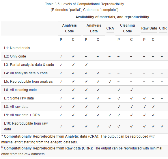
Table 3.5.
You may disagree with some of the levels outlined above, particularly wherever subjective judgment may be required. If so, you are welcome to interpret the levels as unordered categories (independent from their sequence) and suggest improvements using the “Edit” button above (top left corner if you are reading this document in your browser).
Note: The levels suggested here are to be used in the Assessment stage and, optionally, for the Improvement stage. These levels are not meant to be used in the Robustness stage.
3.3.2 Adjusting Levels To Account for Confidential/Proprietary Data
A large fraction of published research in the social sciences uses confidential or proprietary data (e.g., government data from tax records or service provision), generally referred to as administrative data. Since administrative data are rarely readily publicly available, some reproducibility levels presented above only apply once modified. The underlying theme of these modifications is that when data cannot be provided, you can assign a reproducibility score based on the level of detail in the instructions for accessing the data, typically provided in data availability statements (DAS). Use this checklist (.pdf, .md) to guide the assessment, and potential improvement, of a DAS.
When the reproducer cannot directly assess the reproducibility based on publicly available materials, the reproduction package should include certification that a third party (not involved in the paper’s production) faithfully reproduced the results.
Levels 1 and 2 can be applied as described above.
Adjusted Level 3 (L3*): All analysis code is provided, but only partial instructions to access the analysis data are available. This means that the original authors have provided some, but not all, of the following information:
- Contact information, including name of the organization(s) that provides access to at least one individual’s data and contact information.
- Terms of use, including licenses and eligibility criteria for accessing the data, if any.
- Information on data files (meta-data), including the name(s) and number of files, file size(s), relevant file version(s), and number of variables and observations in each file. Though not required, other relevant information may be included, including a dataset dictionary, summary statistics, and synthetic data (fake data with the same statistical properties as the original data).
- Estimated costs for access, including monetary costs such as fees and licenses required to access the data, and non-monetary costs such as wait times and specific geographical locations from where researchers need to access it.
Adjusted Level 4 (L4*): All analysis code is provided, and complete and detailed instructions on how to access the analysis data are available.
Adjusted Level 5 (L5*): All requirements for Level 4* are met, and the authors provide a certification that a third party was able to reproduce the display item (or the paper as a whole) from the analysis data (CRA). Such certification may include a signed letter by a disinterested reproducer or a certificate from a certification agency for data and code (e.g., see CASCaD).
Levels 6 can be applied as described above.
Adjusted Level 7 (7*): All requirements for Level 6* are met, but instructions for accessing the raw data are incomplete. Use the instructions described in Level 3 above to assess the instructions’ completeness.
Adjusted Level 8 (L8*): All requirements for Level 7* are met, and instructions for accessing the raw data are complete.
Adjusted Level 9 (L9*): All requirements for Level 8* are met, and a certification is provided that the display item can be reproduced from the analysis data (CRA).
Adjusted Level 10 (L10*): All requirements for Level 9* are met, and a certification is provided that the display item can be reproduced from the raw data (CRR).
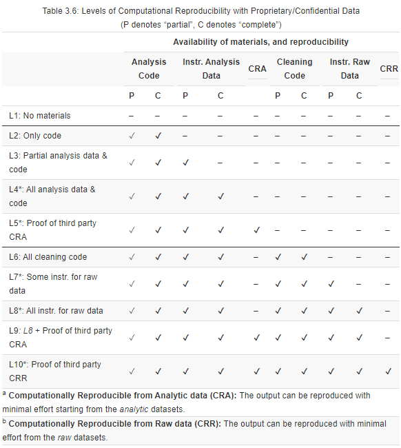
Table 3.6.
3.3.3 Reproducibility dimensions at the paper-level
There are many tools and practices that facilitate the computational reproducibility of the paper as a whole. You can learn more about implementing such reproducibility tools and practices in the Improvements stage, but at this stage, you should only verify whether the current reproduction materials make use of any such tools and practices.
Note: The Assessment stage is the minimum requirement to submit your reproduction. To gain a better understanding of the paper and to help improve the reproducibility of social science research, however, we encourage you to also complete the Improvements and Robustness stages.
a relative location takes the form of
folder_in_rep_materials/sub_folder/file.txt, in contrast to an absolute location that takes the form of/username/documents/projects/repros/folder_in_rep_materials/sub_folder/file.txt↩︎